Dendrogram

1 Introduction

1.1 What is a “Dendrogram”?

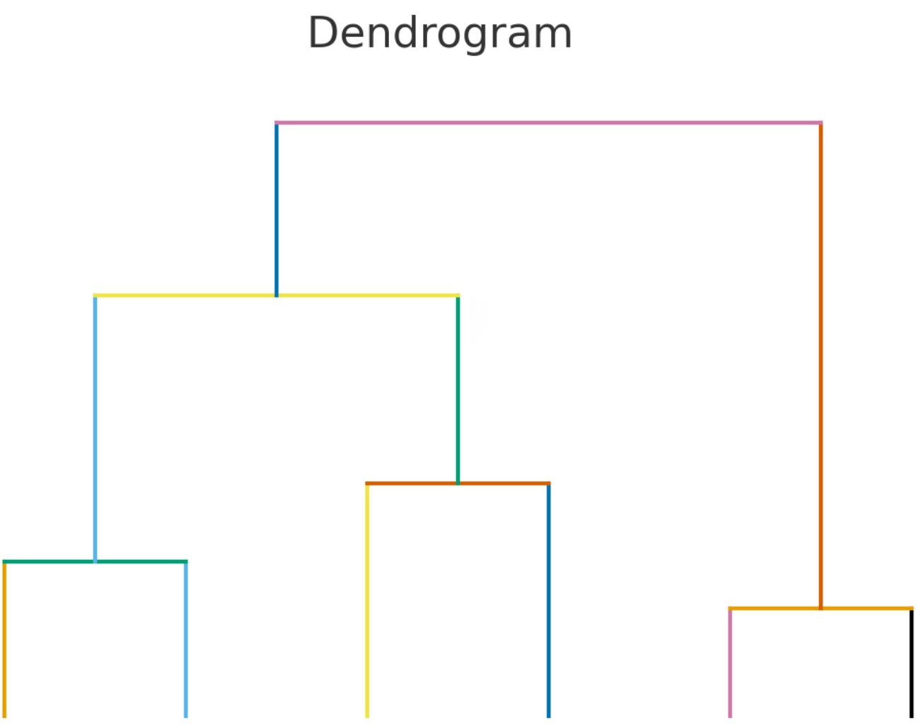
A dendrogram is a tree-like diagram that shows how a set of items group together based on similarity or distance. In computational linguistics, we can use it to visualize how words or dialects relate to each other. Each branch represents a split: items joined lower down the tree are more similar, while those joined higher up are more distant.

When applied to language data, dendrograms give us a way to see clustering patterns — for example, which dialects of Kichwa are most alike (this project!), or how borrowed words differ from native ones. They don’t prove genealogical relationships, but they provide a quick, interpretable snapshot of similarity across datasets.

1.2 The Question

How can we measure similarity between words across dialects?

1.3 The Answer: Levenshtein Distance

The Levenshtein Distance Algorithm (LDA) is a way to measure how different two strings (words, sentences, etc.) are from each other. It does this by counting the minimum number of single-character edits needed to turn one string into the other. The possible edits are:

• Insertion: adding a character
  
• Deletion: removing a character
  
• Substitution: replacing one character with another

Example 1: Orthographic Forms (spelling)
Words for ‘cat’:

• English: cat
  
• Spanish: gato
  
• French: chat
  
• Italian: gatto
  
• German: katze

Pairwise Levenshtein distances (examples):

• cat → gato = 2 edits (insert o, substitute c → g).
  
• cat → chat = 1 edit (insert h after c).
  
• cat → katze = 3 edits (substitute c → k, insert z, insert e).
  
• gato → gatto = 1 edit (insert t).

This already shows some structure — Italian and Spanish are closer, French and English look similar because of orthography (cat/chat), and German is a bit farther.

Example 2: Phonetic Forms (IPA)
Now, let’s compare the same words transcribed in IPA:

• English: /kæt/
  
• Spanish: /ɡato/
  
• French: /ʃa/
  
• Italian: /ɡatto/
  
• German: /katsə/

Pairwise distances (examples):

• /kæt/ → /ʃa/ = 3 edits (substitute k → ʃ, substitute æ → a, delete t).
  
• /ɡato/ → /ɡatto/ = 1 edit (insert t).
  
• /ɡato/ → /katsə/ = 3 edits (substitute ɡ → k, substitute o → ə, insert s).
  
• /kæt/ → /ɡato/ = 3 edits (substitute k → ɡ, substitute æ → a, insert o).
  
• /kæt/ → /katsə/ = 3 edits (substitute æ → a, insert s, insert ə).

Here the picture shifts:

• English and French now look less similar than spelling suggested.
  
• Spanish and Italian remain very close.

Moral of this story
The takeaway here is that while more data usually improves your results, the quality of the data is even more important. Etymological origin matters as well. For example, gato, chat, gatto, cat, and katze all come from the same historical source (cattus in Vulgar Latin). But if you used the Latin word felis instead, the algorithm would see it as very distant — even though historically it refers to the same animal.
Equally, the type of data you use must match your research question:

• If you’re looking at pronunciation similarities, you need IPA transcriptions.
  
• If you’re looking at orthography, then spelling is the right choice.
  
• And if you’re analyzing sentences, alignment becomes critical. Consider:

• English: I want to eat pizza
  
• French: Je veux manger la pizza

To compare properly, you need to align cognates:
I vs Je
want vs veux
eat vs manger
pizza vs pizza

Here, to in English and la in French do not have counterparts. If you leave them in, the algorithm will wrongly compare to with manger and la with eat. You also need to remove punctuation. We don’t want a comma to count in the formula. Also, you want to make sure that if you’re dealing with orthography, all capital letters should be made lowercase (c ≠ C).

1.3.1 Data

We’ll be focusing our work on the Quechuan language family, one of the most widespread and historically significant language families of South America. Quechuan varieties are spoken today by millions of people across the Andes, from Colombia in the north down through Ecuador, Peru, Bolivia, and into parts of Argentina and Chile. Historically, Quechua rose to prominence as the administrative and trade language of the Inca Empire, and after the Spanish conquest it continued to serve as a major lingua franca throughout the region.



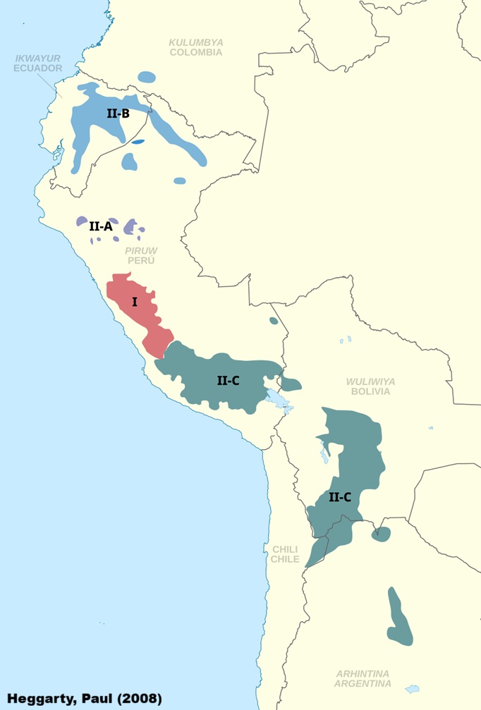
Over time, geographic isolation, contact with Spanish and other Indigenous languages has produced a rich variety of dialects, often differing considerably in vocabulary, sound patterns, and grammar. Linguists typically divide the family into two major branches, Quechua I and Quechua II, with further sub-branches within each. However, not everyone agrees with this classification (see Floyd, 2024). The varieties spoken in Ecuador belong to the Quechua IIB branch, which links them historically to neighbouring Peruvian dialects but also highlights the unique pathways that Ecuadorian Kichwa has taken.



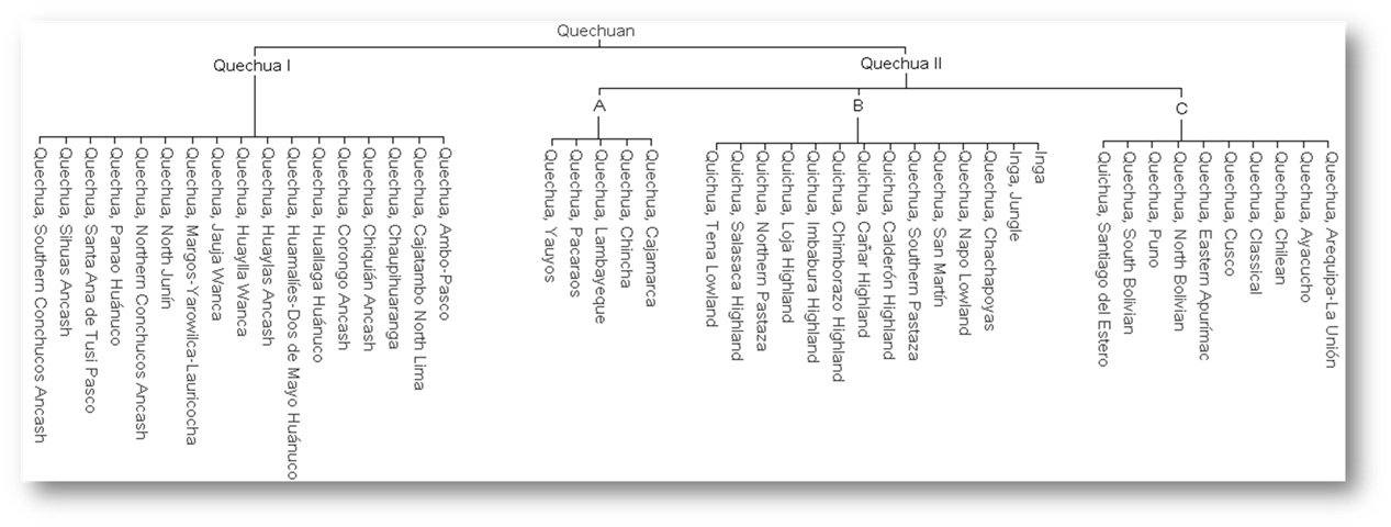
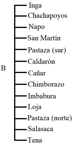
Here we zoom in on one subgroup, Quechua IIB, which includes a number of dialects/languages spoken in Ecuador, Southern Colombia, and northern Peru. This branch is especially important for our purposes, since it contains the Ecuadorian Kichwa varieties we’ll be working with. Alongside these, we’re also including Cuzco Quechua—often treated as the “standard” variety, though in reality it is distinct enough to be considered a separate language—and Unified Kichwa, an artificial standard that was developed in Ecuador for educational and political purposes.



Our data comes via the FEDEPI (2006), which contains the same sentence translated into multiple Ecuadorian dialects. The English translation is The men will come in just two days. We’ll be excluding nearby Colombia and Peruvian dialects/ languages to focus solely on Ecuador, while maintaining Cuzco as a baseline.



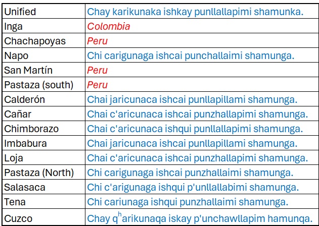
There are a few things to note about this data:

• It’s orthography, not phonetically transcribed. However, aspiration (ʰ) and ejectives (’) are added.
  
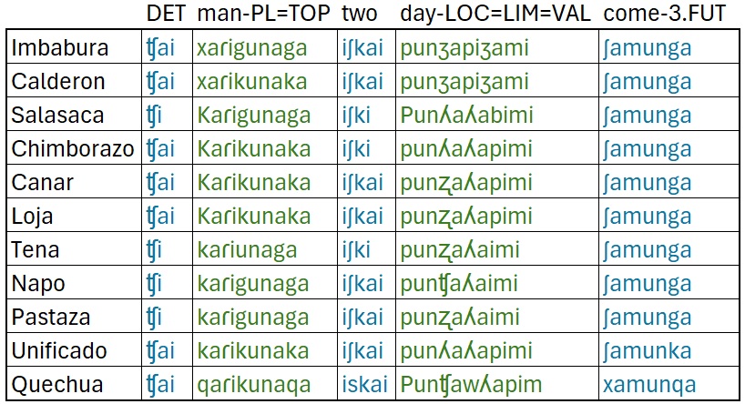
• This sentence was specifically chosen because each word has a direct cognate in each dialect/ language.
  
• The spellings used are based on pronunciation in each region.
  
  
  
  

1.4 Introduction to the Distance Matrix

Up to this point, we’ve looked at examples of how the Levenshtein Distance Algorithm (LDA) works in practice: counting the number of insertions, deletions, or substitutions needed to transform one word into another. But how do we actually calculate this in a systematic way, especially for longer words or whole lists of words?
That’s where the distance matrix comes in.

The idea is simple:
We set up a table with one word across the top and the other word down the side.
Each cell of the table represents the minimum number of edits needed to get from the string on the top to the string on the left.

By filling in the table step by step, we keep track of the ‘cheapest’ (shortest) path of edits at every stage. When we reach the bottom-right corner, we have the Levenshtein distance between the two words.
This method is important because it guarantees that we’ve found the optimal (least costly) sequence of edits, not just a guess. It also makes the algorithm efficient — something that can be scaled up to entire wordlists and then into dendrograms.

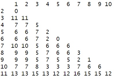
In this example, we’re going to place the Imbabura Kichwa word for ‘men’ (jarikunaka) across the top where each letter has its own column. Then we’ll place the Tena Kichwa word for ‘men’ (cariunaca) vertically (top to bottom) where each letter has its own row. Note that each word begins two row/ columns inwards.
The algorithm: 1. Initialization: 0 → n across the top; 0 → n top to bottom - The top row counts how many insertions you’d need to get from an empty string
- The first column counts how many deletions you’d need to get from the side word to an empty string
2. If the current segments match:
- Copy the number from the diagonal cell (top-left) — no new edit is needed.
3. If they don’t match, look at the three neighbouring (adjacent) cells and take the smallest of those three numbers and add 1.

Once the grid is filled, the bottom-right corner gives the total number of edits (insertions, deletions, substitutions) needed to turn one word into the other.



LDA Video

The we would move on to the next words.
Once complete we would add up the distances from each word as follows:



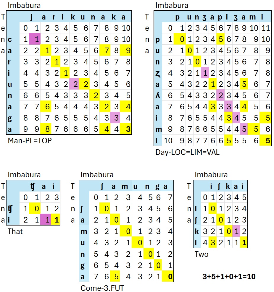
Based on this small dataset, Imbabura Kichwa and Tena Kicwha have a Levenshtien Distance of 9.

1.5 Your turn!

I’ll give you a dialect/ language

Make the following changes Note: I made a few modifications here to make the results more accurate.

• ch → ʧ (so that c and h are a single segment instead of two)
• ay → ai (y at the end of a vowel sequence is /i/.)
• k’ → K (so that k and ' are a single segment instead of two)
• p’ → P (so that p and ' are a single segment instead of two)
• r → ɾ (IPA convention for a tap rather than r which is a trill)
• sh → ʃ (so that s and h are a single segment instead of two)
• ll is ʒ in Imbabura and Calderon
• ll is ʎ elsewhere
• zh → Z is a bit confusing, but likely a retroflex ([ʐ), but as long as we have something ‘different’, that’s all the computer cares about.

Open Excel, do the Matrices for your assigned variety.

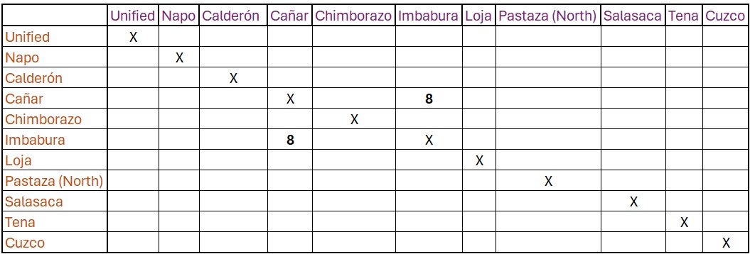
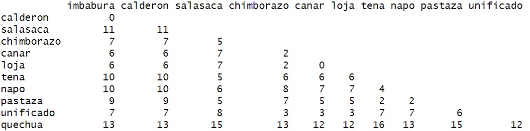
1.6 Dialect/ Language Matrix

The next step is a matrix containing all the languages/ dialects in your data.



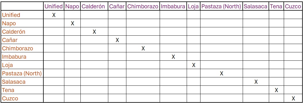
Then we want to enter our distance result from Imbabura and Cañar Kichwa (8)


Next you would go about filling in every language pair, then format it into a string that R can read, before plotting. This would be quite tedious.
To make the computer do this for us, we can use the stringdistmatrix function from the stringdist library.

library(stringdist)

After loading the library, we create a vector where each string under analysis is present between quotes and attached to its associated language.

This will likely mean that we’ll end up with a different value than for the Imbabura-Cañar analysis we just did.

imbabura = "ʧai xaɾikunaka iʃkai punʒapiʒami ʃamunga"
calderon = "ʧai xaɾikunaka iʃkai punʒapiʒami ʃamunga"
salasaca = "ʧi Kaɾigunaga iʃki Punʎaʎabimi ʃamunga"
chimborazo = "ʧai Kaɾikunaka iʃki punʎaʎapimi ʃamunga"
canar = "ʧai Kaɾikunaka iʃkai punʐaʎapimi ʃamunga"
loja = "ʧai Kaɾikunaka iʃkai punʐaʎapimi ʃamunga"
tena = "ʧi kaɾiunaga iʃki punʐaʎaimi ʃamunga"
napo = "ʧi kaɾigunaga iʃkai punʧaʎaimi ʃamunga"
pastaza = "ʧi kaɾigunaga iʃkai punʐaʎaimi ʃamunga"
unificado = "ʧai kaɾikunaka iʃkai punʎaʎapimi ʃamunka"
quechua = "ʧai qaɾikunaqa iskai Punʧawʎapim xamunqa"

The loads the language data transcribed in IPA into a object (vector) with the name of the language variety Each word is spearated by a space (this is necessary).


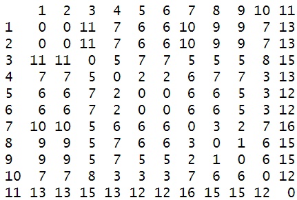
Next, we’re going to use stringdistmatrix, which takes a vector of strings and computes all pairwise string distances between them, returning a square distance matrix (rows and columns = the input strings). Without this, we would have 55 lines of code like this:

stringdist(imbabura, calderon, method='lv')  
stringdist(imbabura, salasaca, method='lv')  
stringdist(imbabura, chimborazo, method='lv')  
stringdist(imbabura, canar, method='lv')  
stringdist(imbabura, loja, method='lv')  
stringdist(imbabura, tena, method='lv')  
stringdist(imbabura, napo, method='lv')  
stringdist(imbabura, pastaza, method='lv')  
stringdist(imbabura, unificado, method='lv')  
stringdist(imbabura, quechua, method='lv')  

stringdist(calderon, salasaca, method='lv')  
stringdist(calderon, chimborazo, method='lv')  
stringdist(calderon, canar, method='lv')  
stringdist(calderon, loja, method='lv')  
stringdist(calderon, tena, method='lv')  
stringdist(calderon, napo, method='lv')  
stringdist(calderon, pastaza, method='lv')  
stringdist(calderon, unificado, method='lv')  
stringdist(calderon, quechua, method='lv')  
stringdist(salasaca, chimborazo, method='lv')  
stringdist(salasaca, canar, method='lv')  
stringdist(salasaca, loja, method='lv')  
stringdist(salasaca, tena, method='lv')  
stringdist(salasaca, napo, method='lv')  
stringdist(salasaca, pastaza, method='lv')  
stringdist(salasaca, unificado, method='lv')  
stringdist(salasaca, quechua, method='lv')  

stringdist(chimborazo,canar, method='lv')  
stringdist(chimborazo,loja, method='lv')  
stringdist(chimborazo,tena, method='lv')  
stringdist(chimborazo,napo, method='lv')  
stringdist(chimborazo,pastaza, method='lv')  
stringdist(chimborazo,unificado, method='lv')  
stringdist(chimborazo,quechua, method='lv')  

stringdist(canar,loja, method='lv')  
stringdist(canar,tena, method='lv')  
stringdist(canar,napo, method='lv')  
stringdist(canar,pastaza, method='lv')  
stringdist(canar,unificado, method='lv')  
stringdist(canar,quechua, method='lv')  

stringdist(loja,tena, method='lv')  
stringdist(loja,napo, method='lv')  
stringdist(loja,pastaza, method='lv')  
stringdist(loja,unificado, method='lv')  
stringdist(loja,quechua, method='lv')  

stringdist(tena,napo, method='lv')  
stringdist(tena,pastaza, method='lv')  
stringdist(tena,unificado, method='lv')  
stringdist(tena,quechua, method='lv')  

stringdist(napo,pastaza, method='lv')  
stringdist(napo,unificado, method='lv')  
stringdist(napo,quechua, method='lv')  

stringdist(pastaza,unificado, method='lv')  
stringdist(pastaza,quechua, method='lv')  

stringdist(unificado,quechua, method='lv')  

A quicker, more effective way to do this would be to combine all the language varieties into a single object and then stringdistmatrix.

lv_data <- c(
    imbabura = "ʧai xaɾikunaka iʃkai punʒapiʒami ʃamunga",
    calderon = "ʧai xaɾikunaka iʃkai punʒapiʒami ʃamunga",
    salasaca = "ʧi Kaɾigunaga iʃki Punʎaʎabimi ʃamunga",
    chimborazo = "ʧai Kaɾikunaka iʃki punʎaʎapimi ʃamunga",
    canar = "ʧai Kaɾikunaka iʃkai punʐaʎapimi ʃamunga",
    loja = "ʧai Kaɾikunaka iʃkai punʐaʎapimi ʃamunga",
    tena = "ʧi kaɾiunaga iʃki punʐaʎaimi ʃamunga",
    napo = "ʧi kaɾigunaga iʃkai punʧaʎaimi ʃamunga",
    pastaza = "ʧi kaɾigunaga iʃkai punʐaʎaimi ʃamunga",
    unificado = "ʧai kaɾikunaka iʃkai punʎaʎapimi ʃamunka",
    quechua = "ʧai qaɾikunaqa iskai Punchawllapim xamunqa"
)

dm <- stringdistmatrix(lv_data, method = "lv")

This reads:
- Create an ‘object’ named lv_data
- ‘combine’ (c()) creates a ‘vector’.
- This is ‘character’ vector because the data are found between quotes ("...")
- This is a ‘named’ character vector because the data has a name (e.g., imbabura =)
- We then use stringdistmatrix to get the Levenshtein distance (lv) from the lv_data object and place it in a matrix table.

Running dm will produce the result.

dm

You’ll notice that there are no names. We’ll need these names for plotting.
The first step will be to convert the data to a data matrix.

dm_mat <- as.matrix(dm)

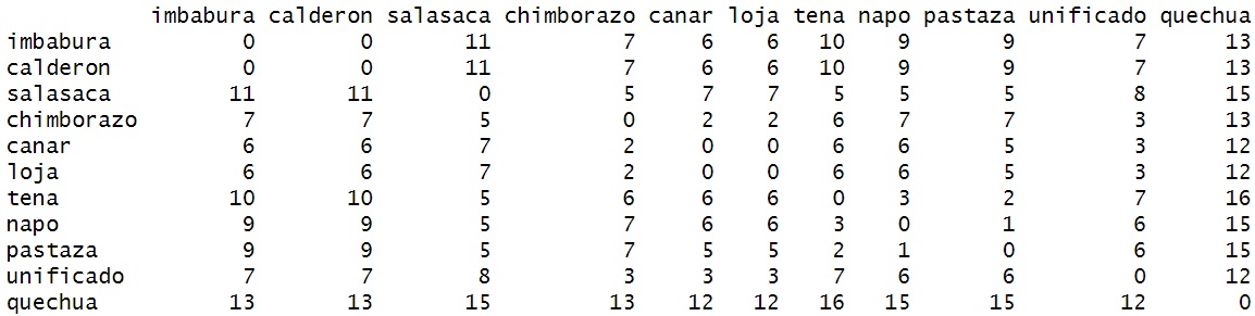
To add them, we’re going to take the names of the character strings from lv_data and place them as both the rows (rownames) and columns (colnames) in the dm_mat object.

rownames(dm_mat) <- names(lv_data)
colnames(dm_mat) <- names(lv_data)

1.7 The Hierarchical Clustering Methods

There are numerous methods for clustering data into a tree structures.
We’re going to review the complete method.

Hierarchical clustering Video

1.8 Doing this with R

This process is obviously laborious. Let’s do this with the computer.
To do this, we’re going to use as.dist (a generic function) to reformat the matrix.

d=as.dist(dm_mat)

• Here, we just remove the duplicate numbers.

After this we, can simply plot the data using R’s built-in plot function.

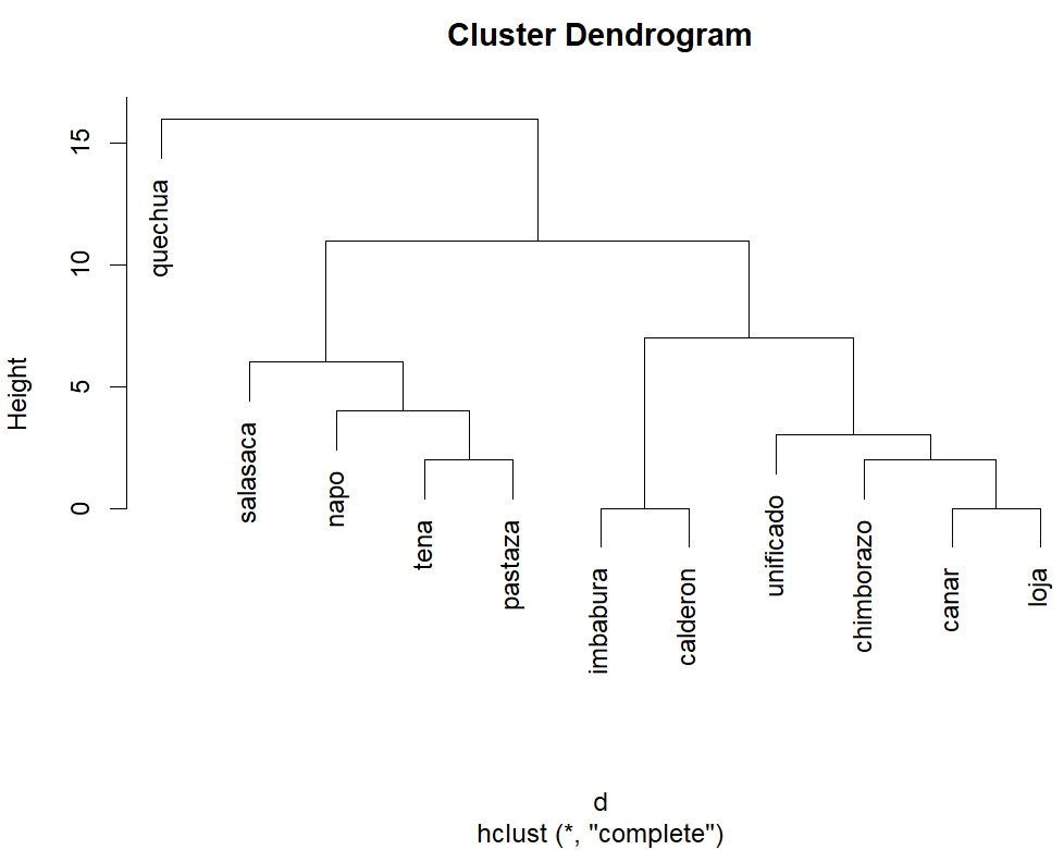
plot(hclust(d,"complete"))

• plot is the generic plotting function in R (not as good as ggplot2, but decent enough)
  
• hclust is the function that actually builds a hierarchical cluster tree (a dendrogram).
  
• d is the dataset we just built.
• "complete" is the linkage method. You can also try “single”, “average”, “ward.D2” etc.
  
  
  
  

Other linking methods, follow different clustering algorithms.

Single linkage (nearest neighbour)

• Distance between clusters = the closest pair of points, one from each cluster.
  

• Tends to make long “chains” of items, because just one close link is enough to join groups.
  
  Complete linkage (furthest neighbour)

• Distance between clusters = the farthest pair of points, one from each cluster.
  

• Produces tight, compact clusters (all members must be fairly close).
  
  Average linkage (UPGMA)

• Distance between clusters = the average of all pairwise distances between points in the two groups.
  

• Balances between single (too loose) and complete (too strict).
  

• Tends to form moderately compact clusters.
  
  Ward’s method (ward.D2)

• Instead of pairwise distances, it looks at the increase in total variance when merging two clusters.
  

• Always chooses the merge that keeps clusters as homogeneous as possible.
  

• Often produces clusters of similar size and shape, popular in many applications.
  
  
  
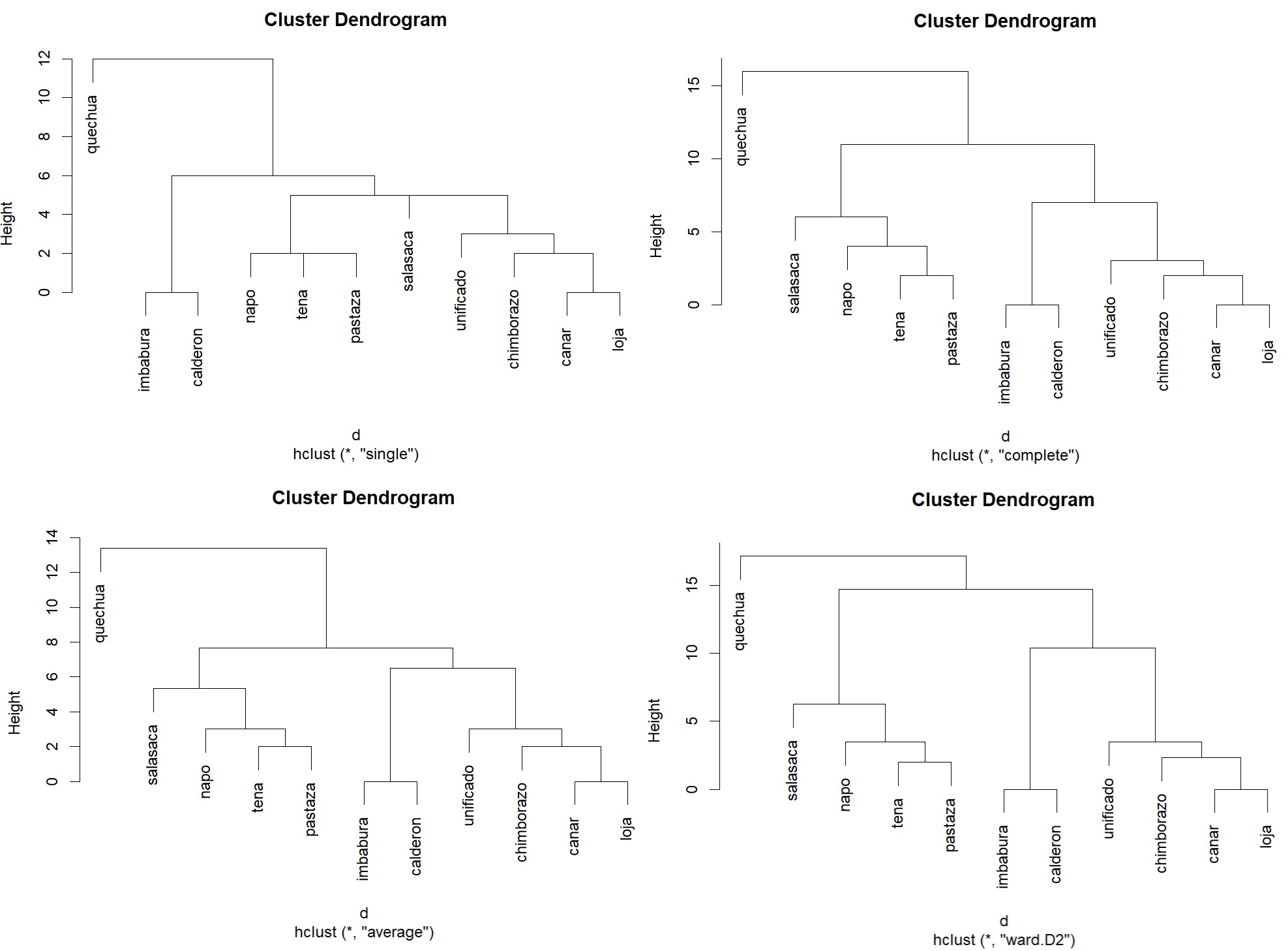
  We can compare these geographically, and get some since of potential accuracy.
  
  
  
  

1.9 Discussion

Obviously, clustering by proximity does not tell the whole story. Ecuador has two major Kichwa groups: Andean Kichwa and Amazonian Kichwa. This broad division is visible in the dendrogram.
Within the Andean region, there are further subdivisions into Northern, Central, and Southern Kichwa. The dendrogram reflects this: Imbabura and Calderon cluster together as northern varieties, while Cañar and Loja group as southern varieties. Chimborazo is a central dialect, but it is often considered closer to the southern group—a relationship also shown in the cluster. We also see that the artificially “unified” (unificado) Standard appears bias towards central-southern Kichwa based on this analysis.
Turning to the Amazonian varieties, the dendrogram using the complete method, places Tena and Pastaza together. This is somewhat surprising, since Tena is in Napo Province, and one might expect it to cluster with Napo. With only a single sentence for comparison, the similarities between Tena and Napo may not have been captured. It is also possible that Tena genuinely shares more with Pastaza than with Napo. Since I do not work directly with these varieties, I cannot say for certain.
The real outlier with the complete method is Salasaca. This variety is generally classified as a central dialect and is expected to align more closely with Chimborazo. Salasaca Kichwa has distinct phonetic patterns and does not fit neatly into the typical structures of other Kichwa dialects. Still, I doubt it is more similar to the Amazonian dialects than to the Andean group.
What this analysis does show is that even with very limited data, we can recover a structure that broadly reflects linguistic reality. With larger samples of text, the results would likely become even more accurate.

1.10 The entire code

library(stringdist)

lv_data <- c(
    Imbabura = "ʧai xaɾikunaka iʃkai punʒapiʒami ʃamunga",
    Calderón = "ʧai xaɾikunaka iʃkai punʒapiʒami ʃamunga",
    salasaca = "ʧi Kaɾigunaga iʃki Punʎaʎabimi ʃamunga",
    Chimborazo = "ʧai Kaɾikunaka iʃki punʎaʎapimi ʃamunga",
    Cañar = "ʧai Kaɾikunaka iʃkai punʐaʎapimi ʃamunga",
    Loja = "ʧai Kaɾikunaka iʃkai punʐaʎapimi ʃamunga",
    Tena = "ʧi kaɾiunaga iʃki punʐaʎaimi ʃamunga",
    Napo = "ʧi kaɾigunaga iʃkai punʧaʎaimi ʃamunga",
    Pastaza = "ʧi kaɾigunaga iʃkai punʐaʎaimi ʃamunga",
    Unificado = "ʧai kaɾikunaka iʃkai punʎaʎapimi ʃamunka",
    Cuzco = "ʧai qaɾikunaqa iskai Punchawllapim xamunqa"
)

dm <- stringdistmatrix(lv_data, method = "lv")

dm_mat <- as.matrix(dm)
rownames(dm_mat) <- names(lv_data)
colnames(dm_mat) <- names(lv_data)

View(dm_mat)

d=as.dist(dm_mat)

plot(hclust(d,"complete"))
plot(hclust(d,"ward.D2"))
plot(hclust(d,"average"))
plot(hclust(d,"single"))

2 HOMEWORK

Translations → Distances → Clusters (Romance)
Download this Excel file Romance

Part A — Build the dataset (58 varieties)
1. Tokenize & label the eight slots (Plus language name):

Language	She	always	close	the	window	before	of	dining
Latin	ea	semper	claudit	XX	fenestram	antequam	XX	cenat
French	ella	toujours	ferme	la	fenêtre	avant	de	dîner

2. Enter cognates per variety. If a slot has no word, write XX (exactly those two letters).

• For example, in the Latin phrase there are no articles or prepositions.
  
• Text to Columns in Excel will help out a bit processing the data.
  
• Don’t “fix” or exclude lexical choices if there’s a translation present (e.g., keep French toujours even if it’s not the direct cognate from Latin (semper).
  • Nerd note: French used to have * sempres, but it’s now obsolete and has been replaced by the contraction of tous les jours ‘all the days’ (toujours). Also, sometimes there are different word orders e.g., ‘always’ comes before ‘close’. When this happens, just move the word to the correct column.
    
    

3. Normalize the data (so distances aren’t inflated by noise): lowercase, trim, keep diacritics, standardize apostrophes. You can do all of this in editPad lite.
   
   
4. Deliverable A: a table with 58 rows × 9 columns (Language name + 8 word slots).
   
   Part B — Manual Levenshtein (French ↔︎ Spanish)
   For each word, show the full matrices for the French tokens vs. the Spanish tokens (8 matrices total).

• Rows = characters of the first word (plus an initial ∅ row).
  
• Columns = characters of the second word (plus an initial ∅ column).
  
• Fill by min(insert, delete, substitute), with substitute cost 0/1.
  
• The bottom-right cell is the distance.
  
• Deliverable B: the 8 completed matrices (no step-by-step ‘narration’ needed, but matrices must be correct). (Yes, this is tedious; that’s the point—you’ll trust the algorithm more after doing it once.)
  
• Your result should look something like this, but obviously for French and Spanish and with 8 matrices.

Part B — Manually Build the fist two clusters Show the steps to build the first two language clusters using the complete method.
For example - Show the matrix.
- Highlight the smallest number minimum number.
- Cluster the language pair in a dendrogram (you can use paint).
- Then merge the language pairs appropriately - Repeat for the next smallest number

Part D — Compute distances & cluster the full set in R
Use the exact tokens you entered (including XX) to keep alignment comparable.
Here’s an example:

lv_data <- c(
   Latin = "ea semper claudit XX fenestram antequam XX cenat",
    French = "elle toujours ferme la fenêtre avant de dîner"
)

A few things to note:
1. The last entry does not end with a comma (,).
2. If a language name has a space, use an underscore (_) instead e.g., Media Lengua → Media_Lengua
3. If a language name has an extended ASCII character (HEX 80 and beyond), you’ll need to change it to standard (HEX 0-7F) character.
4. If you copy directly from Excel into EditPad Lite, you’ll end up with tabs rather than spaces. I don’t know if this will be processed the same (feel free to find out for me), so I would recommend replacing tabs (\t) with spaces ().
5. Make sure there’s no space after the open quote ("), or a space before the closing quote (").
6. There will likely be other errors as you attempt to load the entire dataset into R. You’ll need to figure out what’s causing the error and fix it.

Discuss the results (no more than a paragraph or two)!